
[ad_1]

Making a Higher Dashboard — Fantasy or Actuality?
My beta model 2.0 constructed utilizing Sprint & Plotly as a substitute of Matplotlib
Introduction
In February 2023 I wrote my first Medium submit:
Tips on how to Customise Infographics in Python: Suggestions and Tips
Right here I defined tips on how to create a simplified dashboard with varied diagrams, together with a line plot, pie & bar charts, and a choropleth map. For plotting them I used ‘good outdated’ Matplotlib [1], as a result of I used to be aware of its key phrases and predominant features. I nonetheless imagine that Matplotlib is a superb library for beginning your knowledge journey with Python, as there’s a very massive collective data base. If one thing is unclear with Matplotlib, you’ll be able to google your queries and almost certainly you’ll get solutions.
Nevertheless, Matplotlib might encounter some difficulties when creating interactive and web-based visualizations. For the latter goal, Plotly [2] generally is a good various, permitting you to create uncommon interactive dashboards. Matplotlib, however, is a strong library that gives higher management over plot customization, which is sweet for creating publish-ready visualizations.
On this submit, I’ll attempt to substitute code which makes use of Matlab (1) with that based mostly on Plotly (2). The construction will repeat the preliminary submit, as a result of the sorts of plots and enter knowledge [3] are the identical. Nevertheless, right here I’ll add some feedback on stage of similarity between (1) and (2) for every kind of plots. My predominant intention of writing this text is to look again to my first submit and attempt to remake it with my present stage of information.
Observe: You may be stunned how brief the Plotly code is that’s required for constructing the choropleth map 🙂
However first issues first, and we’ll begin by making a line graph in Plotly.
#1. Line Plot
The road plot generally is a smart selection for displaying the dynamics of adjusting our knowledge with time. Within the case beneath we’ll mix a line plot with a scatter plot to mark every location with its personal shade.
Under yow will discover a code snippet utilizing Plotly that produces a line chart exhibiting the common attendance on the FIFA World Cup over the interval 1990–2018: every worth is marked with a label and a coloured scatter level.
## Line Plot ##

import plotly.graph_objects as go

time = [1990, 1994, 1998, 2002, 2006, 2010, 2014, 2018]
numbers = [48411, 68626, 44676, 42571, 52609, 49499, 53772, 47371]
labels = ['Italy', 'USA', 'France', 'Japan / South Korea', 'Germany',
'South Africa', 'Brazil', 'Russia']

fig = go.Determine()

# Line plot
fig.add_trace(go.Scatter(x=time, y=numbers, mode='strains+markers',
                         marker=dict(shade='black',dimension=10), line=dict(width=2.5)))

# Scatter plot
for i in vary(len(time)):
    fig.add_trace(go.Scatter(x=[time[i]], y=[numbers[i]],
                             mode='markers', identify=labels[i]))

# Format settings
fig.update_layout(title='Common variety of attendees per sport in 1990-2018',
                  xaxis=dict(tickvals=time),
                  yaxis=dict(vary=[35000, 70000]),
                  showlegend=True,
                  legend=dict(x=0.5, y=-0.2),
                  plot_bgcolor='white')

fig.present()
And the outcome seems to be as follows:
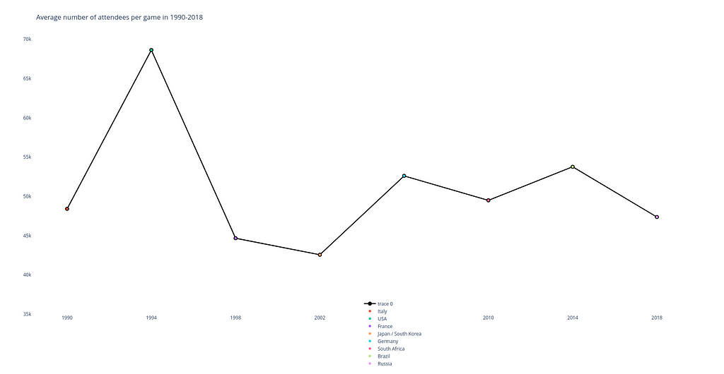
Once you hover your mouse over any level of the chart in Plotly, a window pops up exhibiting the variety of spectators and the identify of the nation the place the event was held.
Degree of similarity to Matplotlib plot: 8 out of 10.
Normally, the code seems to be similar to the preliminary snippet when it comes to construction and the location of the principle code blocks inside it.
What’s completely different: Nevertheless, some variations are additionally introduced. For example, take note of particulars how plot components are declared (e.g. a line plot mode strains+markers which permits to show them concurrently).
What’s essential: For constructing this plot I take advantage of the plotly.graph_objects (which is imported as go) module. It offers an automatically-generated hierarchy of courses referred to as ‘graph objects’ that could be used to characterize varied figures.
#2. Pie Chart (truly, a donut chart)
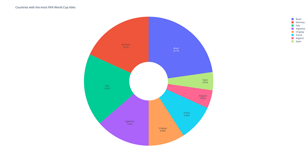
Pie & donut charts are excellent for demonstrating the contributions of various values to a complete quantity: they’re divided in segments, which present the proportional worth of every piece of our knowledge.
Here’s a code snippet in Plotly that’s used to construct a pie chart which might show the proportion between the nations with probably the most World Cup titles.
## Pie Chart ##

import plotly.specific as px

# Knowledge
label_list = ['Brazil', 'Germany', 'Italy', 'Argentina', 'Uruguay', 'France', 'England', 'Spain']
freq = [5, 4, 4, 3, 2, 2, 1, 1]

# Customise colours
colours = ['darkorchid', 'royalblue', 'lightsteelblue', 'silver', 'sandybrown', 'lightcoral', 'seagreen', 'salmon']

# Constructing chart
fig = px.pie(values=freq, names=label_list, title='International locations with probably the most FIFA World Cup titles',
             color_discrete_map=dict(zip(label_list, colours)),
             labels={'label': 'Nation', 'worth': 'Frequency'},
             gap=0.3)

fig.update_traces(textposition='inside', textinfo='p.c+label')
fig.present()
The ensuing visible merchandise is given beneath (by the way in which, it’s an interactive chart too!):
Degree of similarity to Matplotlib plot: 7 out of 10. Once more the code logic is sort of the identical for the 2 variations.
What’s completely different: One may discover that with a assist of gap key phrase it’s potential to show a pie chart right into a donut chart. And see how straightforward and easy it’s to show percentages for every phase of the chart in Plotly in comparison with Matplotlib.
What’s essential: As an alternative of utilizing plotly.graph_objects module, right here I apply plotly.specific module (often imported as px) containing features that may create complete figures directly. That is the easy-to-use Plotly interface, which operates on quite a lot of sorts of knowledge.
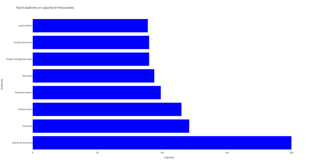
#3. Bar Chart
Bar charts, regardless of whether or not they’re vertical or horizontal, present comparisons amongst completely different classes. The vertical axis (‘Stadium’) of the chart reveals the precise classes being in contrast, and the horizontal axis represents a measured worth, i.e. the ‘Capability’ itself.
## Bar Chart ##

import plotly.graph_objects as go

labels = ['Estádio do Maracanã', 'Camp Nou', 'Estadio Azteca',
          'Wembley Stadium', 'Rose Bowl', 'Estadio Santiago Bernabéu',
          'Estadio Centenario', 'Lusail Stadium']
capability = [200, 121, 115, 99, 94, 90, 90, 89]

fig = go.Determine()

# Horizontal bar chart
fig.add_trace(go.Bar(y=labels, x=capability, orientation='h', marker_color='blue'))

# Format settings
fig.update_layout(title='High-8 stadiums on capability (in 1000's)',
                  yaxis=dict(title='Stadiums'),
                  xaxis=dict(title='Capability'),
                  showlegend=False,
                  plot_bgcolor='white')

fig.present()
Degree of similarity to Matplotlib plot: 6 out of 10.
All in all, the 2 code items have kind of the identical blocks, however the code in Plotly is shorter.
What’s completely different: The code fragment in Plotly is shorter as a result of we don’t have to incorporate a paragraph to position labels for every column — Plotly does this robotically due to its interactivity.
What’s essential: For constructing this sort of plot, plotly.specific module was additionally used. For a horizontal bar char, we are able to use the px.bar perform with orientation=’h’.
#4. Choropleth Map
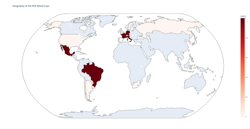
Choropleth map is a superb instrument for visualizing how a variable varies throughout a geographic space. A warmth map is analogous, however makes use of areas drawn in line with a variable’s sample reasonably than geographic areas as choropleth maps do.
Under you’ll be able to see the Plotly code to attract the chorogram. Right here every nation will get its shade relying on the frequency how usually it holds the FIFA World Cup. Darkish crimson nations hosted the event 2 occasions, gentle crimson nations — 1, and all others (grey) — 0.
## Choropleth Map ##

import polars as pl
import plotly.specific as px

df = pl.read_csv('data_football.csv')
df.head(5)
fig = px.choropleth(df, areas='team_code', shade='rely',
                    hover_name='team_name', projection='pure earth',
                    title='Geography of the FIFA World Cups',
                    color_continuous_scale='Reds')
fig.present()
Degree of similarity to Matplotlib plot: 4 out of 10.
The code in Plotly is thrice smaller than the code in Matplotlib.
What’s completely different: Whereas utilizing Matplotlib to construct a choropleth map, we now have to do a number of extra workers, e.g.:
- to obtain a zip-folder ne_110m_admin_0_countries.zip with shapefiles to attract the map itself and to attract nation boundaries, grid strains, and so on.;
- to import Basemap, Polygon and PatchCollection objects from mpl_toolkits.basemap and matplotlib.patches and matplotlib.collections libraries and to make use of them to make coloured background based mostly on the logic we instructed in data_football.csv file.
What’s essential: And what’s the Plotly do? It takes the identical data_football.csv file and with a assist of the px.choropleth perform shows knowledge that’s aggregated throughout completely different map areas or nations. Every of them is coloured in line with the worth of a particular data given, in our case that is the rely variable within the enter file.
As you’ll be able to see, all Plotly codes are shorter (or the identical in a case of constructing the road plot) than these in Matplotlib. That is achieved as a result of Plotly makes it far straightforward to create complicated plots. Plotly is nice for creating interactive visualizations with only a few strains of code.
Sum Up: Making a Single Dashboard with Sprint
Sprint permits to construct an interactive dashboard on a base of Python code without having to be taught complicated JavaScript frameworks like React.js.
Right here yow will discover the code and feedback to its essential components:
import polars as pl
import plotly.specific as px
import plotly.graph_objects as go
import sprint
from sprint import dcc
from sprint import html

external_stylesheets = ['https://codepen.io/chriddyp/pen/bWLwgP.css']

app = sprint.Sprint(__name__, external_stylesheets=external_stylesheets)

header = html.H2(kids="FIFA World Cup Evaluation")

## Line plot with scatters ##

# Knowledge
time = [1990, 1994, 1998, 2002, 2006, 2010, 2014, 2018]
numbers = [48411, 68626, 44676, 42571, 52609, 49499, 53772, 47371]
labels = ['Italy', 'USA', 'France', 'Japan / South Korea', 'Germany', 'South Africa', 'Brazil', 'Russia']

# Constructing chart
chart1 = go.Determine()

chart1.add_trace(go.Scatter(x=time, y=numbers, mode='strains+markers',
                         marker=dict(shade='black',dimension=10), line=dict(width=2.5)))

for i in vary(len(time)):
    chart1.add_trace(go.Scatter(x=[time[i]], y=[numbers[i]],
                             mode='markers', identify=labels[i]))

# Format settings
chart1.update_layout(title='Common variety of attendees per sport in 1990-2018',
                  xaxis=dict(tickvals=time),
                  yaxis=dict(vary=[35000, 70000]),
                  showlegend=True,
                  plot_bgcolor='white')


plot1 = dcc.Graph(
        id='plot1',
        determine=chart1,
        className="six columns"
    )

## Pie chart ##

# Knowledge
label_list = ['Brazil', 'Germany', 'Italy', 'Argentina', 'Uruguay', 'France', 'England', 'Spain']
freq = [5, 4, 4, 3, 2, 2, 1, 1]

# Customise colours
colours = ['darkorchid', 'royalblue', 'lightsteelblue', 'silver', 'sandybrown', 'lightcoral', 'seagreen', 'salmon']

# Constructing chart
chart2 = px.pie(values=freq, names=label_list, title='International locations with probably the most FIFA World Cup titles',
             color_discrete_map=dict(zip(label_list, colours)),
             labels={'label': 'Nation', 'worth': 'Frequency'},
             gap=0.3)

chart2.update_traces(textposition='inside', textinfo='p.c+label')

plot2 = dcc.Graph(
        id='plot2',
        determine=chart2,
        className="six columns"
    )

## Horizontal bar chart ##

labels = ['Estádio do Maracanã', 'Camp Nou', 'Estadio Azteca',
          'Wembley Stadium', 'Rose Bowl', 'Estadio Santiago Bernabéu',
          'Estadio Centenario', 'Lusail Stadium']
capability = [200, 121, 115, 99, 94, 90, 90, 89]

# Constructing chart
chart3 = go.Determine()

chart3.add_trace(go.Bar(y=labels, x=capability, orientation='h', marker_color='blue'))

# Format settings
chart3.update_layout(title='High-8 stadiums on capability (in 1000's)',
                  yaxis=dict(title='Stadiums'),
                  xaxis=dict(title='Capability'),
                  showlegend=False,
                  plot_bgcolor='white')


plot3 = dcc.Graph(
        id='plot3',
        determine=chart3,
        className="six columns"
    )

## Chropleth map ##

# Knowledge
df = pl.read_csv('data_football.csv')

# Constructing chart
chart4 = px.choropleth(df, areas='team_code', shade='rely',
                    hover_name='team_name', projection='pure earth',
                    title='Geography of the FIFA World Cups',
                    color_continuous_scale='Reds')

plot4 = dcc.Graph(
        id='plot4',
        determine=chart4,
        className="six columns"
    )


row1 = html.Div(kids=[plot1, plot2],)
row2 = html.Div(kids=[plot3, plot4])
format = html.Div(kids=[header, row1, row2], type={"text-align": "middle"})

app.format = format

if __name__ == "__main__":
    app.run_server(debug=False)
Feedback to the code:
- First, we have to import all libraries (together with HTML modules) and initialize dashboard with a assist of the string app = sprint.Sprint(__name__, external_stylesheets=external_stylesheets).
- We then paste every graph into Sprint core parts to additional combine them with different HTML parts (dcc.Graph). Right here className=”six columns” wants to make use of half the display for every row of plots.
- After that we create 2 rows of html.Div parts with 2 plots in every. As well as, a easy CSS with the type attribute can be utilized to show the header of our dashboard within the format string. This format is ready because the format of the app initialized earlier than.
- Lastly, the final paragraph permits to run the app regionally (app.run_server(debug=False)). To see the dashboard, simply comply with the hyperlink http://127.0.0.1:8050/ and you’ll discover one thing just like the picture beneath.
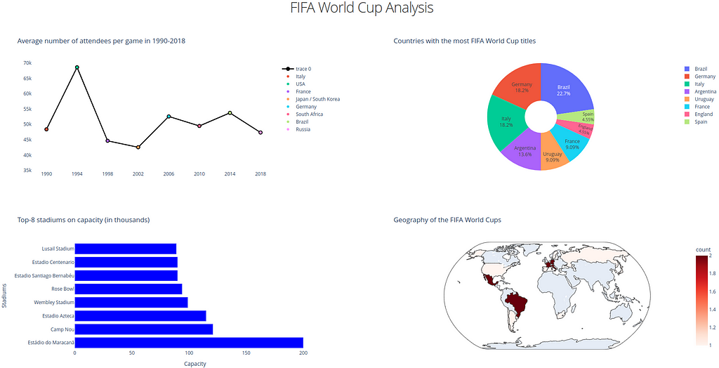
Remaining Remarks
Truthfully, the query within the title was rhetorical, and solely you, expensive reader, can determine whether or not the present model of the dashboard is healthier than the earlier one. However at the very least I attempted my greatest (and deep inside I imagine that model 2.0 is healthier) 🙂
You might assume that this submit doesn’t include any new data, however I couldn’t disagree extra. By scripting this submit, I needed to emphasise the significance of bettering abilities over time, even when the primary model of the code might not look that dangerous.
I hope this submit encourages you to have a look at your completed initiatives and attempt to remake them utilizing the brand new methods accessible. That’s the predominant cause why I made a decision to substitute Matplotlib with Plotly & Sprint (plus the latter two make it straightforward to create knowledge evaluation outcomes).
The power to continuously enhance your work by bettering an outdated model or utilizing new libraries as a substitute of those you used earlier than is a superb talent for any programmer. If you happen to take this recommendation as a behavior, you will note progress, as a result of solely follow makes excellent.
And as at all times, thanks for studying!
References
- The primary web page of Matplotlib library: https://matplotlib.org/secure/
- The primary web page of Plotly library: https://plotly.com/python/
- Fjelstul, Joshua C. “The Fjelstul World Cup Database v.1.0.” July 8, 2022. https://www.github.com/jfjelstul/worldcup
Creating a greater dashboard — delusion or actuality? was initially printed in In the direction of Knowledge Science on Medium, the place persons are persevering with the dialog by highlighting and responding to this story.
[ad_2]